LOTKA-VOLTERRA MODEL
The Lotka-Volterra model is a classic system dynamics predator-prey model that will achieve equilibrium. As the predator population rises, prey population falls, leading to the fall of the predator population and maintaining the equilibrium of the system. In this model, prey and predators are represented as stocks. The Prey stock has FLOWS for births and deaths, while the Predator stock has FLOWS for eating and deaths. This model contains a submodel, “Lotka-Volterra Chip” with SIX inputs that control initial stock values, prey births and deaths, and predator eating and deaths. Each of the submodel inputs can be adjusted using Sliders. The predator-prey outputs are shown on two graphs, one that shows the periodic values over time and a second that shows the phase shift.
The Lotka–Volterra equations, also known as the predator–prey equations, are a pair of first-order, non-linear, differential equations frequently used to describe the dynamics of biological systems in which two species interact, one as a predator and the other as prey. The populations change through time according to a pair of equations:
Standard Lotka-Volterra equations.
dx/dt = x(α−βy)
dy/dt = −y(γ−δx)
(x represents size of prey population; y represents size of predator population):
Equations used by this version of the Lotka-Volterra model:
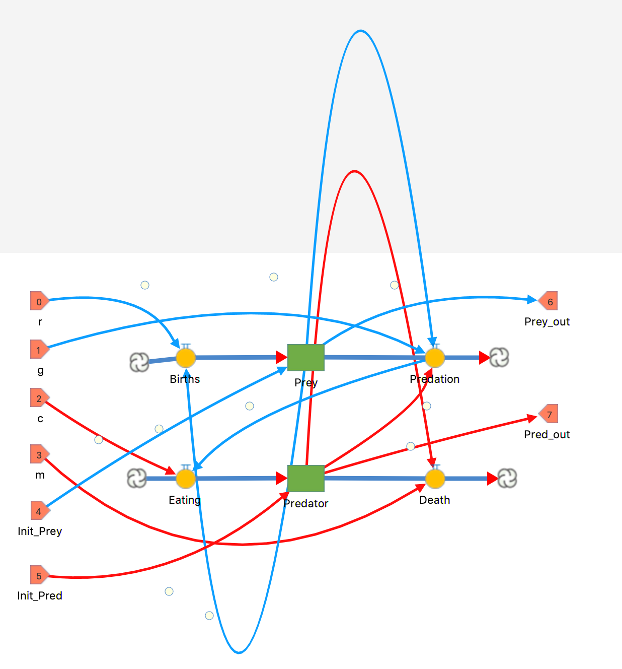
dPrey/dt = r⋅Prey−g⋅Pred⋅Prey
dPred/dt = c⋅g⋅Pred⋅Prey−m⋅Pred
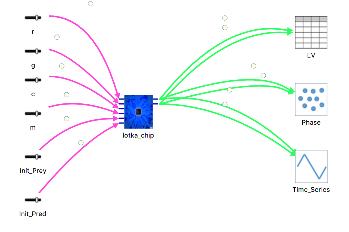
This model makes use of Numerus' submodel/chip capability to hide the details of the model at a lower level.
THE MODEL:
We have called the bottom layer "Lotka" and the top layer "Lotka_Demo." Always make sure to distinguish layers if you have more than one.
THE BOTTOM LAYER:
THE TOP LAYER:
In this model, we want to point out a few components:
1. As mentioned earlier, Sliders assist in allowing the user to adjust values. Therefore, the user can observe how a model behaves with various values of our sliders above. They are represented as the black lines with a little white bar that can be moved. We will demonstrate this in further detail after Launching this model.
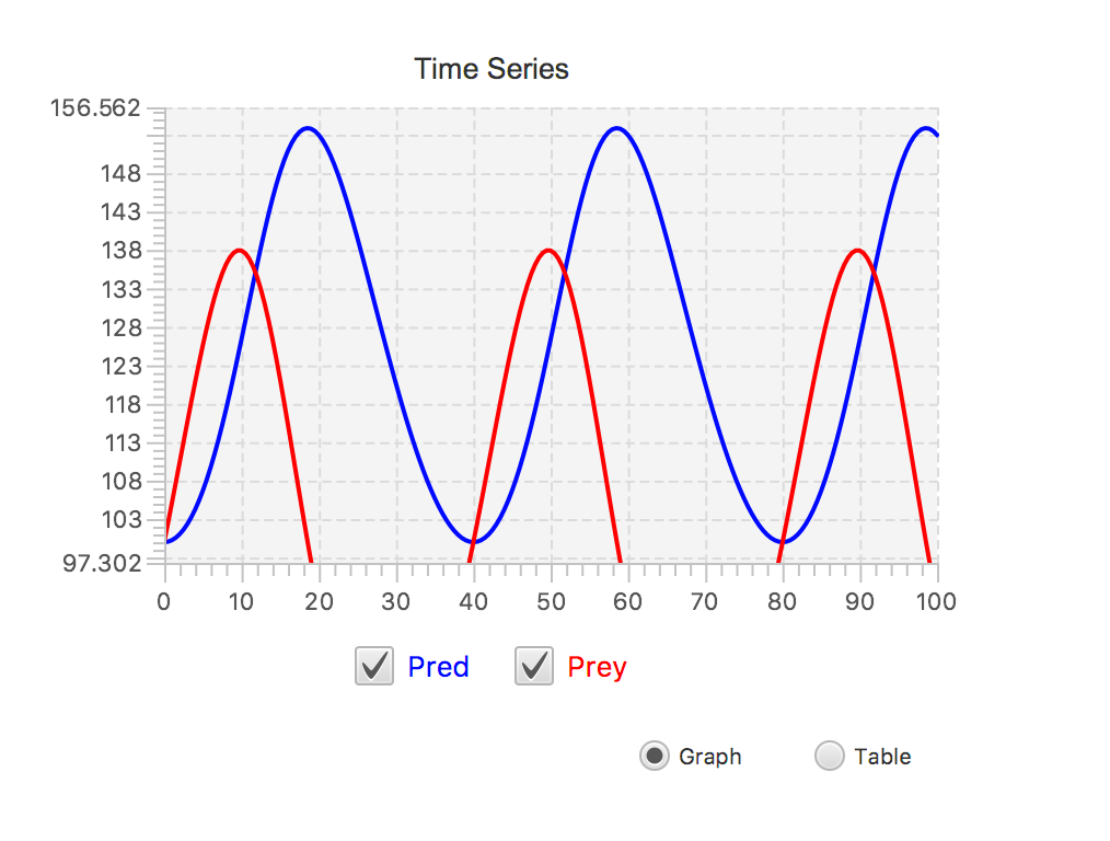
2. Time_Series is represented by a Line Graph. You may find this in Displays & Controls >> LineGraph.
3. Phase is represented by a Scatter Chart. You may find this in Displays & Controls >> ScatterChart.
4. LV is represented by a Table. You may find this in Displays & Controls >> Table.
THE LAUNCH:
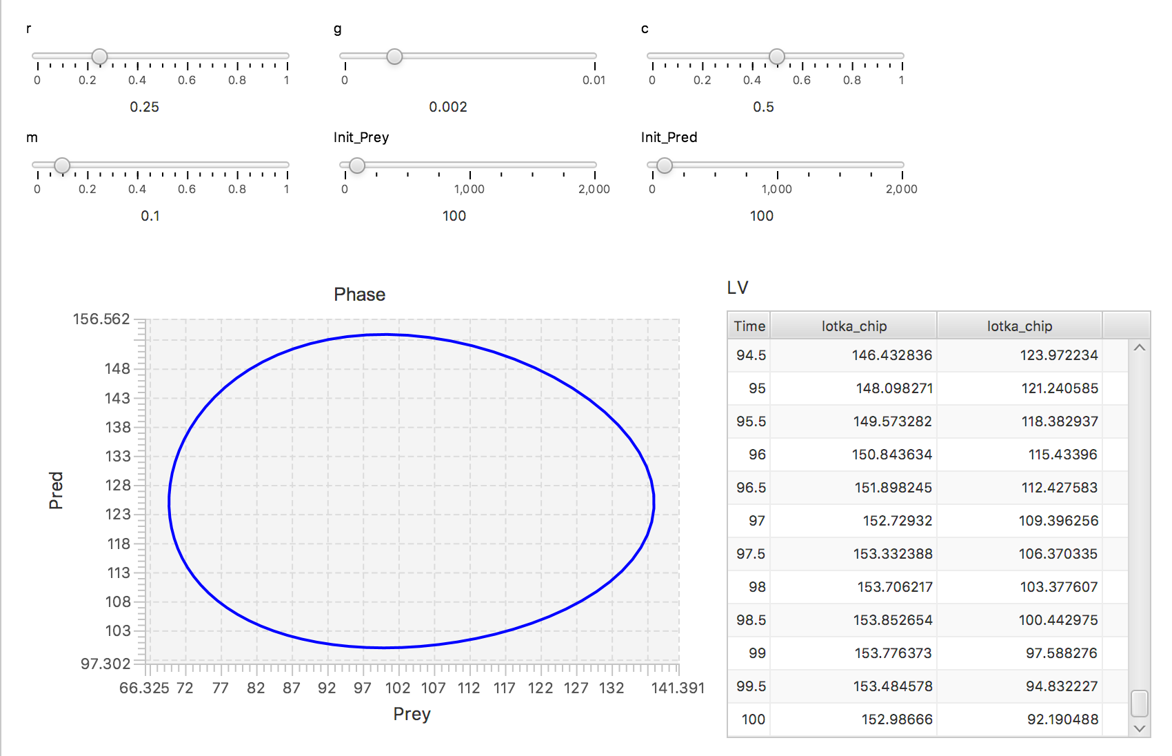
Make note of the sliders above: r, g, c, m, Init_Prey, and Init_Pred. Those bubbles on the lines can be clicked on, and dragged across the bar, to change the respective values.